This vignette provides an in-depth walk-through of the
MRPWorkflow and MRPModel classes in the
shinymrp package. You will find practical information
about the purpose, arguments, and caveats of each method, enabling you
to conduct MRP analyses programmatically.
For an introduction to the package and workflow concepts, begin with the Getting started with shinymrp vignette.
Initializing the workflow
MRP analysis begins by instantiating an MRPWorkflow
object with mrp_workflow(). The object-oriented design
efficiently manages your data and supports a reproducible workflow
without requiring repeated user input. All workflow methods are accessed
via the R6 $
operator.
library(shinymrp)
workflow <- mrp_workflow()
1. Data preparation
MRP requires two key data components:
- Sample data: Your analysis sample, which must include the outcome of interest (binary or continuous) and predictors (demographic, geographic, etc.), such as COVID-19 test records or survey responses.
- Poststratification data: A table containing population sizes of groups defined by demographic and geographic factors.
For details on accepted formats and preprocessing, see the Data Preprocessing vignette.
1.1 Preprocessing the sample data
Sample data should be a tidy data frame with your outcome measure and predictors. Time-varying data are also supported, allowing dates or indices (e.g., week, month, or year) to be incorporated for time-varying summaries and estimates.
The example_sample_data() function demonstrates accepted
structures and common options:
- whether a time variable is included
- whether the data are aggregated
- whether the data follow a specific standard (e.g., medical records from the Epic system)
- whether the outcome measure is binary (modeled with binomial distributions) or continuous (modeled with Gaussian/normal distributions)
sample_data <- example_sample_data(
  is_timevar = TRUE,
  is_aggregated = TRUE,
  special_case = NULL,
  family = "binomial"
)
head(sample_data)
#> # A tibble: 6 × 10
#>     zip sex    race  age    time county state date       total positive
#>   <dbl> <chr>  <chr> <chr> <dbl>  <dbl> <dbl> <date>     <dbl>    <dbl>
#> 1 71354 female black 0-17      3  22025    22 2020-01-13     1        0
#> 2 71354 female black 0-17      5  22025    22 2020-01-27     1        1
#> 3 71354 female black 0-17      9  22025    22 2020-02-24     1        0
#> 4 71354 female black 18-34     1  22025    22 2019-12-30     2        1
#> 5 71354 female black 18-34     6  22025    22 2020-02-03     1        0
#> 6 71354 female black 18-34     9  22025    22 2020-02-24     1        1
Data preprocessing is performed with the $preprocess()
method, which standardizes formats (e.g., recodes age groups, creates
time indices), removes duplicates, and prepares data for modeling.
Note: Only basic cleaning is performed. Conduct preliminary data checks beforehand.
workflow$preprocess(
  sample_data,
  is_timevar = TRUE,
  is_aggregated = TRUE,
  special_case = NULL,
  family = "binomial"
)
#> Preprocessing sample data...
1.2 Assembling poststratification data
1.2.1 Linking to ACS
Use the $link_acs() method to retrieve
poststratification data from the American Community Survey (ACS),
specifying the desired geographic level and reference year (i.e., the
last year of the five-year ACS data collection). Supported levels
include ZIP code, county, and state. If not specified,
poststratification data are aggregated for the U.S. population.
workflow$link_acs(link_geo = "zip", acs_year = 2021)
#> Linking data to the ACS...
1.2.2 Importing custom poststratification data
You can also import your own poststratification data using
$load_pstrat(). Requirements
mirror those for sample data.
pstrat_data <- example_pstrat_data()
workflow$load_pstrat(pstrat_data, is_aggregated = TRUE)
#> Preprocessing poststratification data...
2. Descriptive statistics
The MRPWorkflow class provides methods for creating
visualizations of demographic distributions, geographic coverage, and
outcome summaries.
Use $demo_bars() to generate bar plots comparing
demographic distributions in the sample and poststratification data.
workflow$demo_bars(demo = "sex")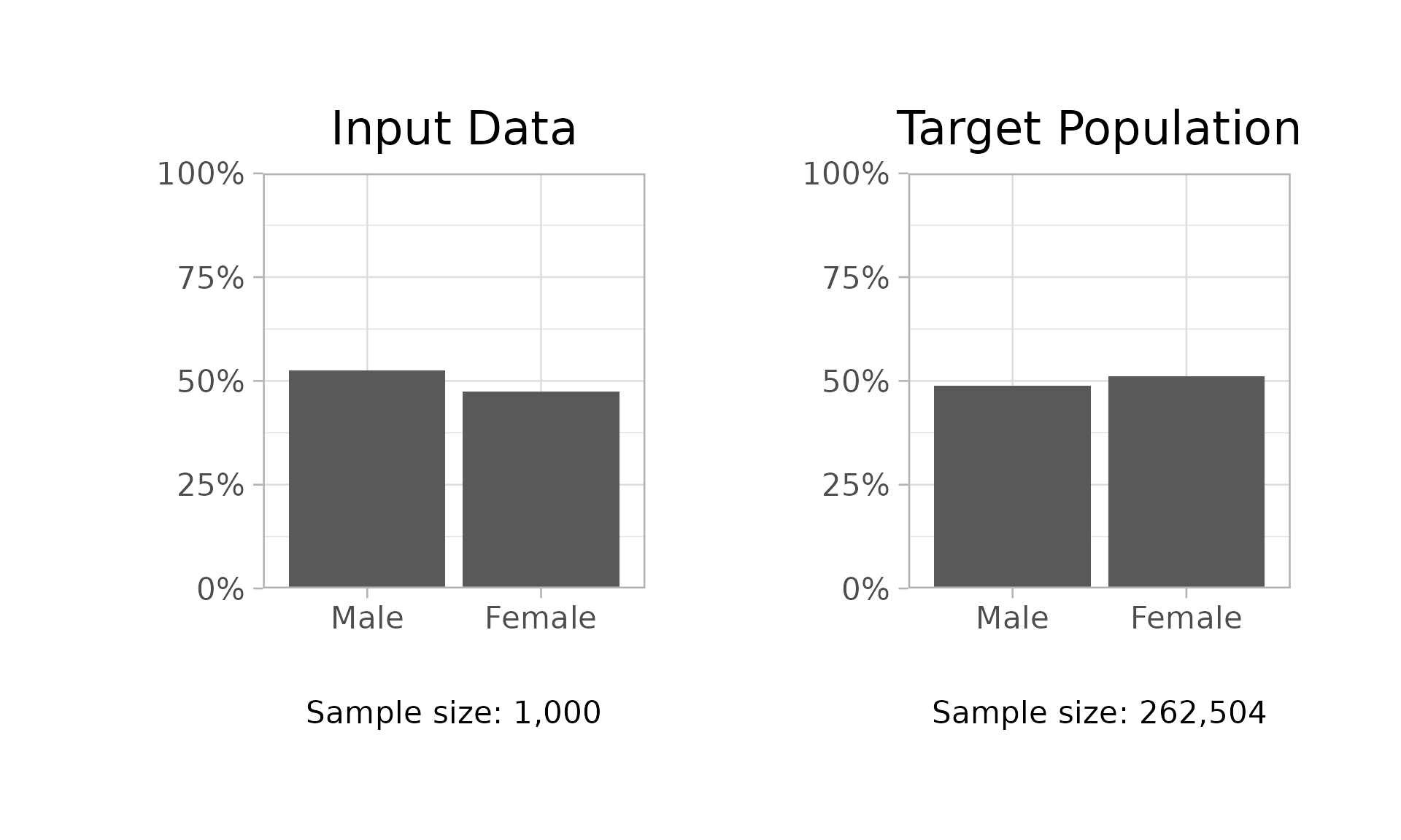
For analyzing COVID-19 test data with linked geographic predictors,
the $covar_hist() method creates frequency histograms of
the geographic predictors. This method will give the following error if
it is called with incompatible data that do not include geographic
predictors.
workflow$covar_hist(covar = "income")
#> Error in workflow$covar_hist(covar = "income"): Covariate data is not available. This method is only available for COVID data.
$sample_size_map() visualizes sample sizes across
geographic areas in an interactive choropleth map, powered by highcharter.
workflow$sample_size_map()
#> Registered S3 method overwritten by 'quantmod':
#>   method            from
#>   as.zoo.data.frame zoo
$outcome_plot() creates plots of average outcome values,
including time variation if present.
workflow$outcome_plot()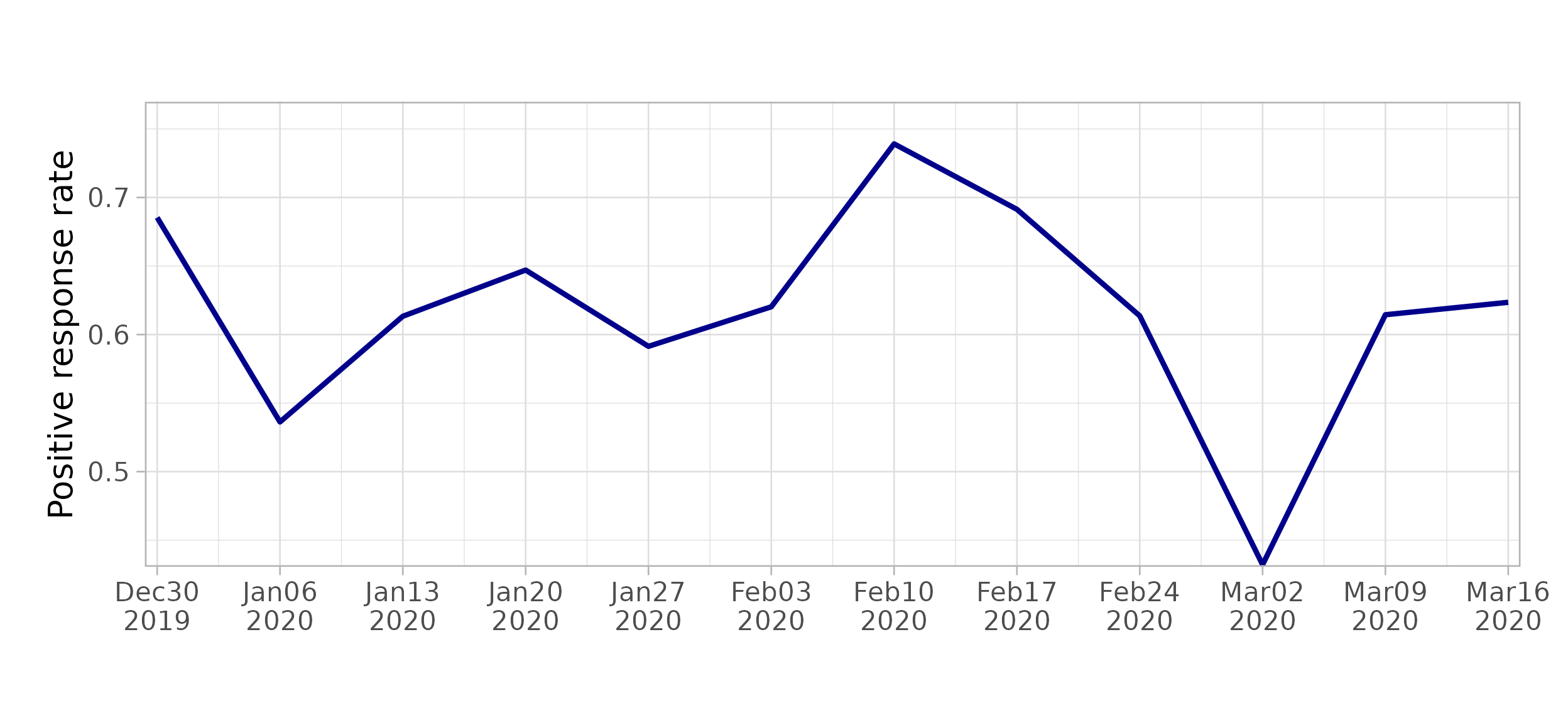
$outcome_map() visualizes outcome summaries by
geography, with options for the maximum or minimum value across
time.
workflow$outcome_map(summary_type = "max")3. Model building
The MRPModel class is a wrapper around CmdStanR objects,
providing a high-level interface for obtaining posterior summaries and
diagnostics.
3.1 Model specification
Use $create_model() to specify the model, including the
mean structure (fixed and varying effects, two-way interactions) and
priors. Varying effects assume normal distributions with unknown
standard deviations (with specified priors). Stan code is generated for
compilation via CmdStanR. Supported prior types include:
normal(mu, sigma)student_t(nu, mu, sigma)-
structured(see Si et al., 2020) -
icar(see Besag et al., 1991) -
bym2(see Riebler et al., 2016)
Default priors are used if "" (empty string) is
supplied:
- Overall intercept: normal(0, 5)
- Coefficient: normal(0, 3)
- Standard deviation (main effect): normal+(0, 3)
- Standard deviation (interaction): normal+(0, 1)
3.2 Model fitting
The $fit() method runs Stan’s main Markov chain Monte
Carlo algorithm via CmdStanR.
model1$fit(
  n_iter = 500,
  n_chains = 2,
  seed = 123,
  show_messages = FALSE,
  show_exceptions = FALSE
)
#> Warning: 1 of 500 (0.0%) transitions ended with a divergence.
#> See https://mc-stan.org/misc/warnings for details.
3.3 Posterior summaries and diagnostics
The fitted MRPModel object extracts draws from the
internal CmdStanMCMC object for summaries and
diagnostics.
-
Posterior summary and convergence diagnostics: Use
$summary()for posterior statistics, effective sample sizes, and R-hat diagnostics.
model1$summary()
#> $fixed
#>              Estimate Est.Error    l-95% CI  u-95% CI     R-hat Bulk_ESS
#> intercept  -0.1552038 0.2029703 -0.51179360 0.2636422 1.0015135 155.1940
#> sex.male    0.2824838 0.1338178  0.02599781 0.5476556 0.9973944 621.5216
#> race.black         NA        NA          NA        NA        NA       NA
#> race.other  0.7682242 0.1672083  0.45840460 1.0993380 0.9987605 456.4001
#> race.white  0.8251199 0.1669716  0.50039767 1.1567253 0.9999359 348.4526
#>            Tail_ESS
#> intercept  148.2918
#> sex.male   421.2527
#> race.black       NA
#> race.other 366.2108
#> race.white 395.3222
#>
#> $varying
#>                   Estimate Est.Error   l-95% CI  u-95% CI    R-hat Bulk_ESS
#> age (intercept)  0.2687213 0.1887081 0.02469051 0.7533799 1.021851 123.6085
#> time (intercept) 0.2716189 0.1202040 0.07451838 0.5388200 1.005514 159.8250
#>                  Tail_ESS
#> age (intercept)  192.4378
#> time (intercept) 159.7993
#>
#> $residual
#> data frame with 0 columns and 0 rows
#>
#> $spatial_proportion
#> data frame with 0 columns and 0 rows-
Additional diagnostics: Use
$diagnostics()for detailed diagnostic information about the MCMC process.
model1$diagnostics()
#>               Metric
#> 1         Divergence
#> 2 Maximum tree depth
#> 3             E-BFMI
#>                                                       Message
#> 1         1 of 500 (0.2%) transitions ended with a divergence
#> 2 0 of 500 transitions hit the maximum tree depth limit of 10
#> 3 0 of 2 chains had an E-BFMI less than 0.3-
Posterior predictive check: Use
$pp_check()to compare posterior predictive samples against observed data.
workflow$pp_check(model1)
#> Running posterior predictive check...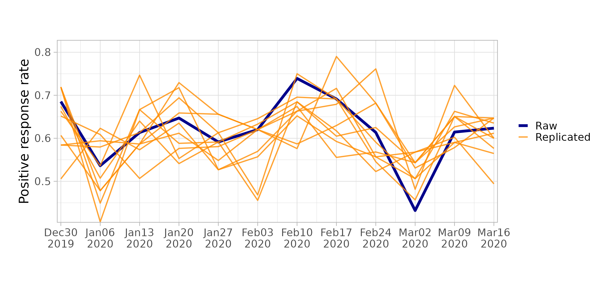
-
Model comparison: Compare models via leave-one-out
cross-validation with
$compare_models().
model2 <- workflow$create_model(
  intercept_prior = "normal(0, 4)",
  fixed = list(
    sex = "normal(0, 2)",
    race = "normal(0, 2)"
  ),
  varying = list(
    age = "",
    time = ""
  ),
  interaction = list(
    `age:time` = "normal(0, 1)",
    `race:time` = "normal(0, 1)",
    `sex:time` = "normal(0, 1)"
  )
)

model2$fit(
  n_iter = 500,
  n_chains = 2,
  seed = 123,
  show_messages = FALSE,
  show_exceptions = FALSE
)
workflow$compare_models(model1, model2)
#> Running leave-one-out cross-validation...
#>        elpd_diff  se_diff
#> model2  0.000000 0.000000
#> model1 -1.637057 2.601372
3.4 Saving and loading models
You can easily save and restore models using the qs2
package. The $save() gathers all posterior draws and
diagnostics, then calls qs2::qs_save() internally.
model1$save(file = "model1.qs2")

# load back into workspace
model1 <- qs2::qs_read("model1.qs2")
4. Result visualization
Use $estimate_plot() to visualize the model estimates,
either overall or by group, with a 95% credible interval by default.
Users can specify alternative intervals.
workflow$estimate_plot(model1, group = "sex", interval = 0.95)
#> Running poststratification...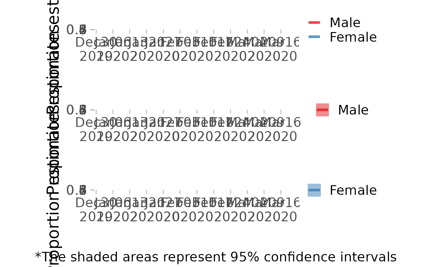
For time-varying data, $estimate_map() creates snapshots
of geography-based estimates at specific time points.
time_index is irrelevant for cross-sectional data.
workflow$estimate_map(model1, geo = "county", interval = 0.95, time_index = 1)