MRPWorkflow objects

A MRPWorkflow object is an R6 object created by the mrp_workflow() function. This class provides methods for all steps in the workflow, from data preparation and visualization to model fitting.

Methods

MRPWorkflow objects have the following associated methods with their own (linked) documentation pages:

Data preparation

Method	Description
$preprocess()	Preprocess sample data.
$preprocessed_data()	Return preprocessed sample data.
$link_acs()	Link sample data to ACS data.
$load_pstrat()	Load custom poststratification data.

Model fitting & diagnostics

Method	Description
$create_model()	Create a MRPModel object.
$pp_check()	Perform posterior predictive check.
$compare_models()	Compare models using LOO-CV.

Visualization

Method	Description
$demo_bars()	Create demographic comparison bar plots.
$covar_hist()	Create geographic covariate distribution histograms.
$sample_size_map()	Create sample size map.
$outcome_plot()	Create summary plots of raw outcome measure.
$outcome_map()	Visualize raw outcome measure by geography.
$estimate_plot()	Visualize estimates for demographic groups.
$estimate_map()	Visualize estimates for geographic areas.

Examples

 # \donttest{
   library(shinymrp)

   # Initialize the MRP workflow
   workflow <- mrp_workflow()

   # Load example data
   sample_data <- example_sample_data()

   ### DATA PREPARATION

   # Preprocess sample data
   workflow$preprocess(
     sample_data,
     is_timevar = TRUE,
     is_aggregated = TRUE,
     special_case = NULL,
     family = "binomial"
   )
#> Preprocessing sample data...

   # Link data to the ACS
   # and obtain poststratification data
   workflow$link_acs(
     link_geo = "zip",
     acs_year = 2021
   )
#> Linking data to the ACS...

   ### DESCRIPTIVE STATISTICS

   # Visualize demographic distribution of data
   sex_bars <- workflow$demo_bars(demo = "sex")

   # Visualize geographic distribution of data
   ss_map <- workflow$sample_size_map()
#> Registered S3 method overwritten by 'quantmod':
#>   method            from
#>   as.zoo.data.frame zoo 

   # Visualize outcome measure
   raw_outcome_plot <- workflow$outcome_plot()

   ### MODEL BUILDING

   # Create new model objects
   model <- workflow$create_model(
     intercept_prior = "normal(0, 4)",
     fixed = list(
       sex = "normal(0, 2)",
       race = "normal(0, 2)"
     ),
     varying = list(
       age = "",
       time = ""
     )
   )

   # Run MCMC
   model$fit(n_iter = 500, n_chains = 2, seed = 123)
#> Running MCMC with 2 parallel chains, with 1 thread(s) per chain...
#> 
#> Chain 1 Iteration:   1 / 500 [  0%]  (Warmup) 
#> Chain 2 Iteration:   1 / 500 [  0%]  (Warmup) 
#> Chain 1 Iteration:  50 / 500 [ 10%]  (Warmup) 
#> Chain 2 Iteration:  50 / 500 [ 10%]  (Warmup) 
#> Chain 1 Iteration: 100 / 500 [ 20%]  (Warmup) 
#> Chain 1 Iteration: 150 / 500 [ 30%]  (Warmup) 
#> Chain 2 Iteration: 100 / 500 [ 20%]  (Warmup) 
#> Chain 1 Iteration: 200 / 500 [ 40%]  (Warmup) 
#> Chain 2 Iteration: 150 / 500 [ 30%]  (Warmup) 
#> Chain 1 Iteration: 250 / 500 [ 50%]  (Warmup) 
#> Chain 1 Iteration: 251 / 500 [ 50%]  (Sampling) 
#> Chain 2 Iteration: 200 / 500 [ 40%]  (Warmup) 
#> Chain 1 Iteration: 300 / 500 [ 60%]  (Sampling) 
#> Chain 2 Iteration: 250 / 500 [ 50%]  (Warmup) 
#> Chain 2 Iteration: 251 / 500 [ 50%]  (Sampling) 
#> Chain 1 Iteration: 350 / 500 [ 70%]  (Sampling) 
#> Chain 2 Iteration: 300 / 500 [ 60%]  (Sampling) 
#> Chain 2 Iteration: 350 / 500 [ 70%]  (Sampling) 
#> Chain 1 Iteration: 400 / 500 [ 80%]  (Sampling) 
#> Chain 2 Iteration: 400 / 500 [ 80%]  (Sampling) 
#> Chain 1 Iteration: 450 / 500 [ 90%]  (Sampling) 
#> Chain 2 Iteration: 450 / 500 [ 90%]  (Sampling) 
#> Chain 1 Iteration: 500 / 500 [100%]  (Sampling) 
#> Chain 2 Iteration: 500 / 500 [100%]  (Sampling) 
#> Chain 1 finished in 1.1 seconds.
#> Chain 2 finished in 1.1 seconds.
#> 
#> Both chains finished successfully.
#> Mean chain execution time: 1.1 seconds.
#> Total execution time: 1.3 seconds.
#> 
#> Warning: 1 of 500 (0.0%) transitions ended with a divergence.
#> See https://mc-stan.org/misc/warnings for details.

   # Estimates summary and diagnostics
   model$summary()
#> $fixed
#>              Estimate Est.Error    l-95% CI  u-95% CI     R-hat Bulk_ESS
#> intercept  -0.1552038 0.2029703 -0.51179360 0.2636422 1.0015135 155.1940
#> sex.male    0.2824838 0.1338178  0.02599781 0.5476556 0.9973944 621.5216
#> race.black         NA        NA          NA        NA        NA       NA
#> race.other  0.7682242 0.1672083  0.45840460 1.0993380 0.9987605 456.4001
#> race.white  0.8251199 0.1669716  0.50039767 1.1567253 0.9999359 348.4526
#>            Tail_ESS
#> intercept  148.2918
#> sex.male   421.2527
#> race.black       NA
#> race.other 366.2108
#> race.white 395.3222
#> 
#> $varying
#>                   Estimate Est.Error   l-95% CI  u-95% CI    R-hat Bulk_ESS
#> age (intercept)  0.2687213 0.1887081 0.02469051 0.7533799 1.021851 123.6085
#> time (intercept) 0.2716189 0.1202040 0.07451838 0.5388200 1.005514 159.8250
#>                  Tail_ESS
#> age (intercept)  192.4378
#> time (intercept) 159.7993
#> 
#> $other
#> data frame with 0 columns and 0 rows
#> 

   # Sampling diagnostics
   model$diagnostics()
#>               Metric
#> 1         Divergence
#> 2 Maximum tree depth
#> 3             E-BFMI
#>                                                       Message
#> 1         1 of 500 (0.2%) transitions ended with a divergence
#> 2 0 of 500 transitions hit the maximum tree depth limit of 10
#> 3                   0 of 2 chains had an E-BFMI less than 0.3

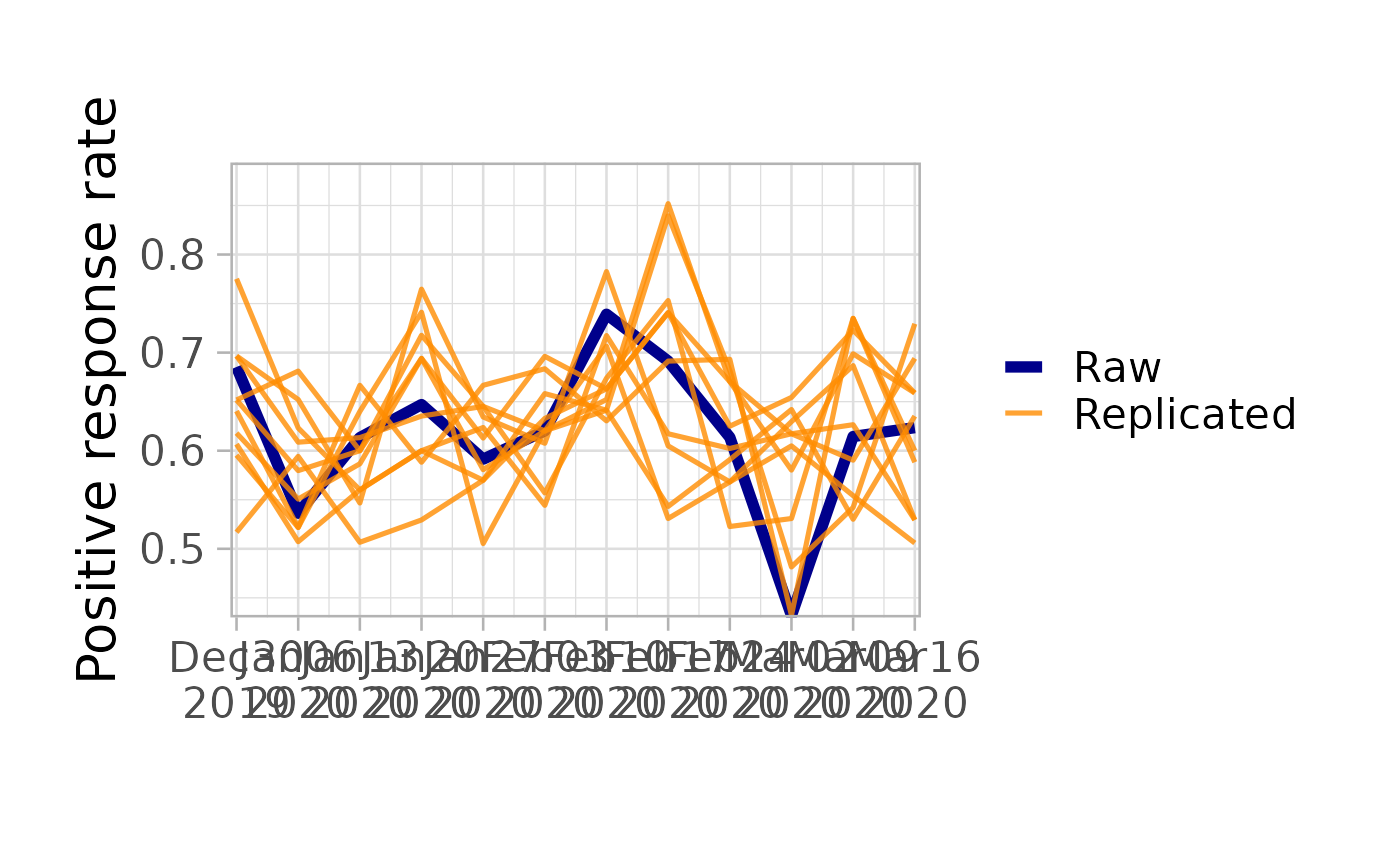
   # Posterior predictive check
   workflow$pp_check(model)
#> Running posterior predictive check...


   ### VISUALIZE RESULTS

   # Plots of overall estimates, estimates for demographic groups, and geographic areas
   workflow$estimate_plot(model, group = "sex")
#> Running poststratification...


   # Choropleth map of estimates for geographic areas
   workflow$estimate_map(model, geo = "county")

 # }